
Quantum State K designs
In this article I am going to tell you what quantum k-designs. Although they are a relatively niche area of research in quantum information, I really found them an amazing concept and I thought that you may enjoy reading about them as well.
You can find this article published in Imperial College Physics Review, a student-led scientific magazine.
Qubits and wave functions
Before digging into k-designs, we need to review a couple of concepts. You may have heard about quantum computing and the special information element that they use: the qubit. When I talk about a qubit, I want you to imagine an atom with an electron that can be in an excited or ground state. Physicists love to make up new notation and in this context they call them respectively $|0\rangle$ and $|1\rangle$; the fact that $\vert0\rangle$ represents the excited state is a matter of convention. Alternatively, they write them as $|g\rangle$ and $|e\rangle$ (they do love making up notation) [1, p. 38].
The magic of quantum mechanics resides in the fact that the electron doesn’t need to occupy only the ground or the excited state of the atom, but it can be in a superposition of both at the same time (the famous Schrödinger’s cat!). Generally, we would write the wavefunction of the electron as:
\[|\psi\rangle = a \vert 0\rangle + b \vert 1\rangle\]However, when you measure the “excitedness” of the electron, you find it either in the excited or in the ground state, never in both! It would be quite spooky to see Schrödinger’s cat both alive and dead at the same time. Mathematically, this derives from the fact that the states $\vert 0\rangle$ and $\vert 1\rangle$ are orthogonal. All wavefunctions and states of a particular system (such as our qubit) live in a world (space) called Hilbert space $\mathcal{H}$. [1, p. 21]
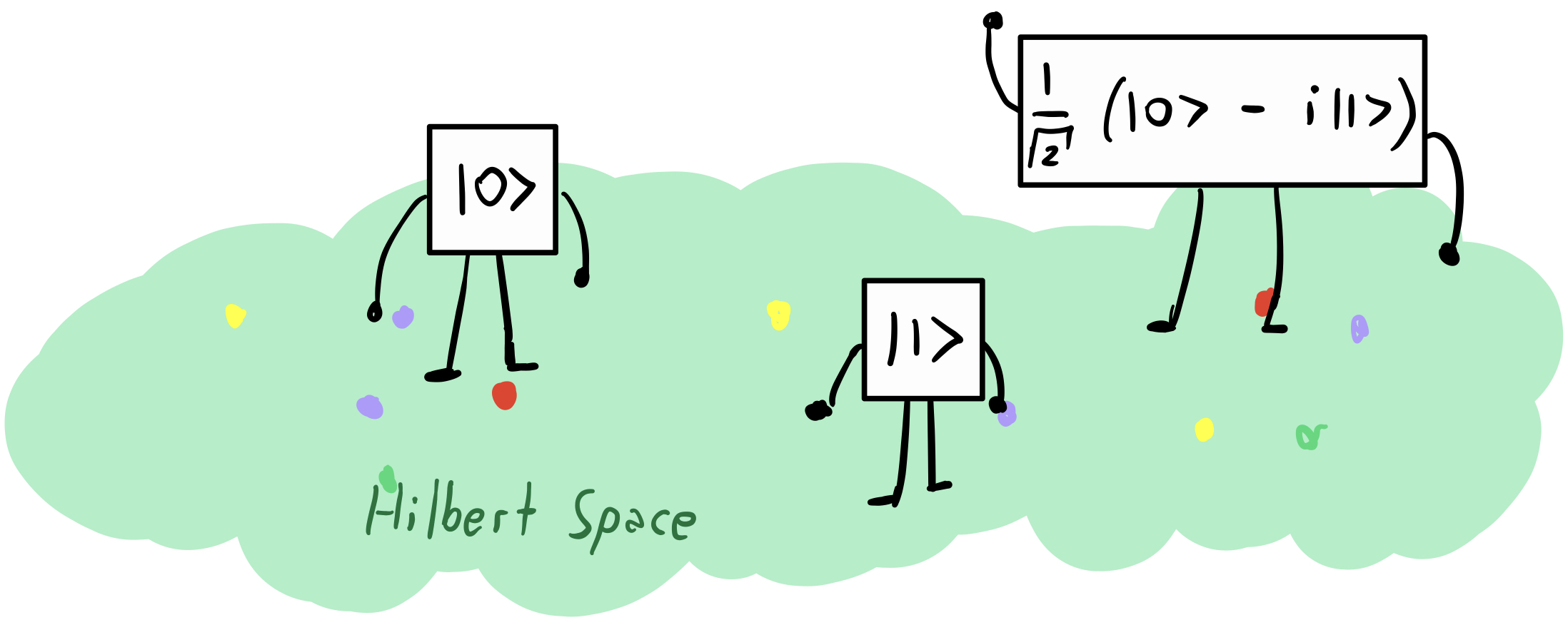
Ensembles
If we take a bunch of states that live in the Hilbert space and we put them into a set, we can make an ensemble [2]:
\[\{|\phi_i\rangle\},\qquad |\phi_i\rangle \in \mathcal{H}\quad i = 1,2,...,N\]We can be more general, and attribute to each of the $N$ states in the ensemble a probability $p_i$ such that the sum of all the probabilities adds to 1. This is quite of an arbitrary step: we are really free to choose the probability at our own pleaure. Then, we can write:
\[\{(\vert\phi_i\rangle, p_i)\}\qquad |\phi_i\rangle \in \mathcal{H},\quad \sum_{i=1}^N p_i = 1\]and this is still an ensemble [2].
Polynomial of a quantum state
We quickly reviewed what states are, and we saw that we can collect a bunch of them into an ensemble. It may seem a bit underwhelming, but the whole definition of quantum state k-design revolves around the concept of polynomial. Before telling me that you already know everything about them, allow me to tell you this: you can define a function $g(|\psi\rangle)$ that is a polynomial and that takes a wavefunction as an input. If you are half as bamboozled as I was when I first read this, allow me to give you an example.
Quantum computers use quantum technology to transform one state in the Hilbert space into another. These steps are called quantum gates. Experimentalists want to make sure that their quantum computer is working correctly and they compare the wavefunction they obtain after transformation with the output they expect. One metric to evaluate how close two wavefunctions are is called Fidelity and it is a number between $1$ (the two states are identical) and $0$ (you definitely need to fix your machine) [1].
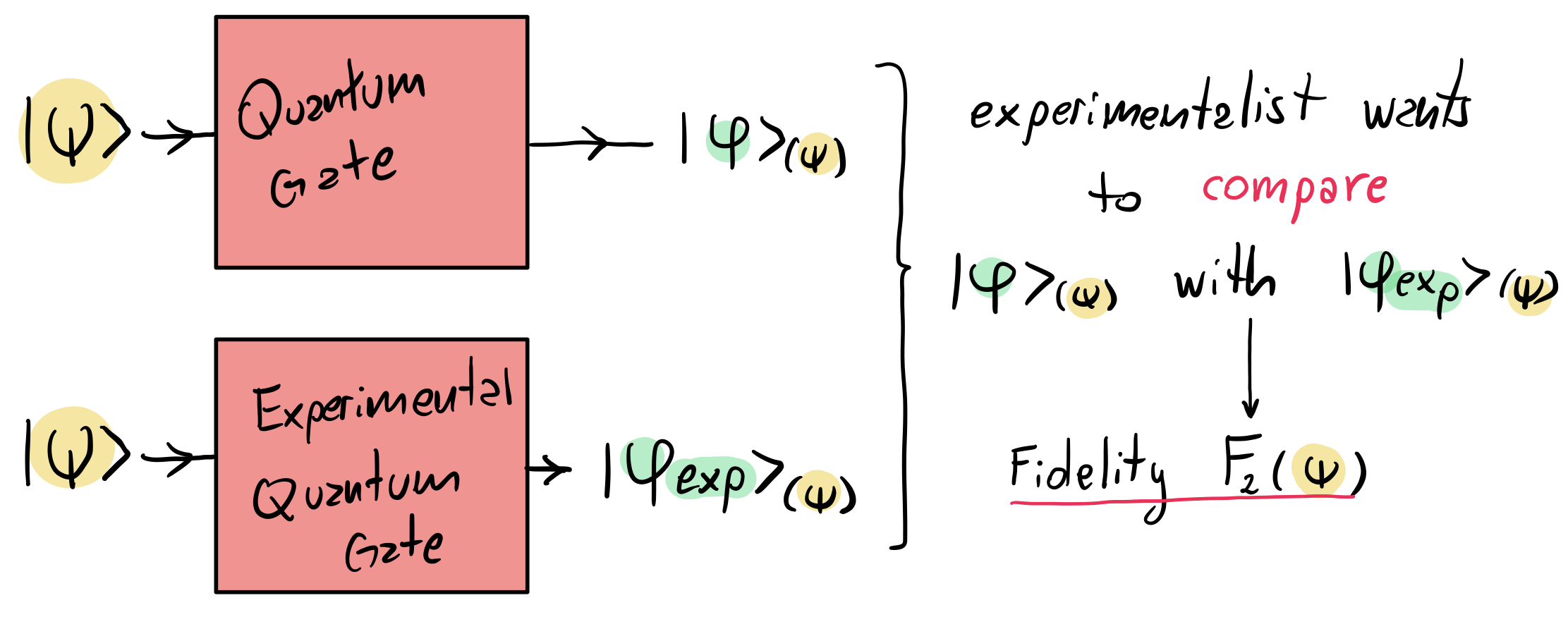
Following the diagram above, for every input wavefunction $\vert\psi\rangle$ we can find the output state of the experiment and evaluate the fidelity with the expected state. All this process can be described by the fidelity function $F_2(\vert\psi\rangle)$ that takes an input state $\vert\psi\rangle$ as its argument. The function $F_2(\vert\psi\rangle)$ involves squaring the wavefunction and therefore it turns out to be a polynomial of order 2, which motivates the subscript I added [2].
Quantum state k-designs
Now we have all the ingredients to talk about quantum k-designs. Say that our friend experimentalist wants to evaluate the average fidelity $F_2$ for the gate they implemented. They should find the expectation value of $F_2(\vert\psi\rangle)$ over all possible states that populate the Hilbert space $\mathcal{H}$. Mathematically, we would write this as:
\[\int_{\mathcal H}F_2(\vert\psi\rangle)\ d\vert\psi\rangle\]Seing the expression above, the experimentalist would probably burst into tears. The poor scientist would have to run infinitely many experiments to exactly evaluate the average value of the fidelity $\langle F_2\rangle$!
However, here comes the magic. For the case of a second order polynomial, it is enough for the experimentalist to evaluate the function $F_2$ for all states $\vert\phi_i\rangle$ that belong to a special ensemble \(\{(\vert\phi_i\rangle, p_i)\}\) that we call quantum state 2-design. Then, they can compute the average value of $F_2$ by doing [3]:
\[\langle F_2\rangle = \sum_{i} p_i F_2(\vert\phi_i\rangle)\]This is amazing! We converted an impossible problem into a sum over a finite number of quantum states, which is something possible to do! What’s even more puzzling is that the same special ensemble can be used to find the expectation value of any second order polynomial $g_2(\vert\psi\rangle)$, not just $F_2$! Furthermore, the existence of these quantum state k-design ensembles is always guaranteed for any polynomial order $k$ and for any Hilbert space $\mathcal H$. However, finding the expression of these particular ensembles may be a tricky endeavour. If you want to read more into the mathematical proofs, you can check out these references [2][3].
To rephrase all of this more generally, a quantum k-design is a special ensemble, such that the average of any polynomial $g_k$ of order $k$ taken over all the states that populate the Hilbert space, can be computed by performing a sum over the states in the ensemble weighted by their probabilities. This is encapsulated by this equality:
\[\int_{\mathcal H}g_k(\vert\psi\rangle)\ d\vert\psi\rangle = \sum_{i} p_i g_k(\vert\phi_i\rangle)\qquad \mathrm{for}\ \{(\vert\phi_i\rangle, p_i)\}\ \mathrm{a\ k\ design}\]Since this is super abstract, I wanted to conclude by showing you a picture of quantum k-designs in the case of a single qubit [3-5].
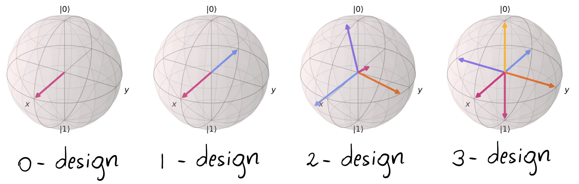
The spheres are called Bloch sphere and they are a practical way of visualising all the possible states populating the Hilbert space of a qubit. You can think about each point on the surface of the sphere as corresponding to a different state $\vert\psi\rangle$. The arrows in one sphere represent the states in a k-design ensemble \(\{(\vert\phi_i\rangle, p_i)\}\), in which we have taken the probabilities $p_i$ to be the same. As the order of k increases, more vectors appear in the sphere, and they better cover all the surface. Hence, the k-design gets more and more representative of the totality of the Hilbert space!
It is this feature of compressing the Hilbert space into few, distributed states that makes k-design useful in fields such as quantum hardware benchmarking and quantum cryptography. To sum up, I hope you found this topic as fascinating as I do, and next time you see your experimentalist friend working on an impossible task, I hope you will direct them to this article on k-designs !
[1] P. Kaye et al. An introduction to quantum computing, Oxford university press (2007)
[2] Martin Adam, Applications of Unitary k-designs in Quantum Information Processing, Master thesis (2013)
[3] https://pennylane.ai/qml/demos/tutorial_unitary_designs.html
[4] Emergent Randomness and Benchmarking from Many-Body Quantum Chaos
[5] A. Ketter et al. Entanglement characterization using quantum designs, Quantum, volume 4, page 325, arXiv:2004.08402v3, (2020)